Plotting Walkthrough
This tutorial walks through the standard plotting tools you'll use after
generating a synthetic ensemble. The synhydro.plotting module provides
ensemble-aware versions of the common diagnostic figures (timeseries with
percentile bands, flow duration curves, monthly distributions, and a
multi-panel validation summary), all sharing a consistent argument style.
For the full list of plotting functions and their arguments see the Plotting API reference.
Setup
Generate a small Kirsch ensemble that we can re-use for every plot below. 20 realizations is enough to make percentile bands meaningful while keeping the example fast.
import synhydro
from synhydro.plotting import (
    plot_timeseries,
    plot_flow_duration_curve,
    plot_monthly_distributions,
    plot_validation_panel,
)

Q_daily = synhydro.load_example_data()
Q_monthly = Q_daily.resample("MS").sum()
site = Q_monthly.columns[0]

gen = synhydro.KirschGenerator()
gen.fit(Q_monthly)
ensemble = gen.generate(n_realizations=20, n_years=20, seed=42)
Every plot below takes the ensemble as its first positional argument and
returns a (fig, ax) (or (fig, axes)) tuple, so you can compose them into
larger figures or save them to disk via filename=....
Timeseries with observed overlay
plot_timeseries shows the ensemble median, a 10th-90th percentile band,
and optionally a few member traces, with the observed series overlaid for
reference.
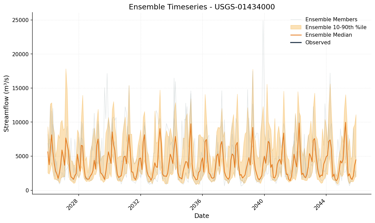
Use start_date and end_date to zoom into a sub-window, or log_scale=True
for highly-skewed flows.
Flow duration curve
plot_flow_duration_curve plots non-exceedance probability vs flow on a log
y-axis. The shaded band is the inter-realization range; the dashed line is
the observed FDC.
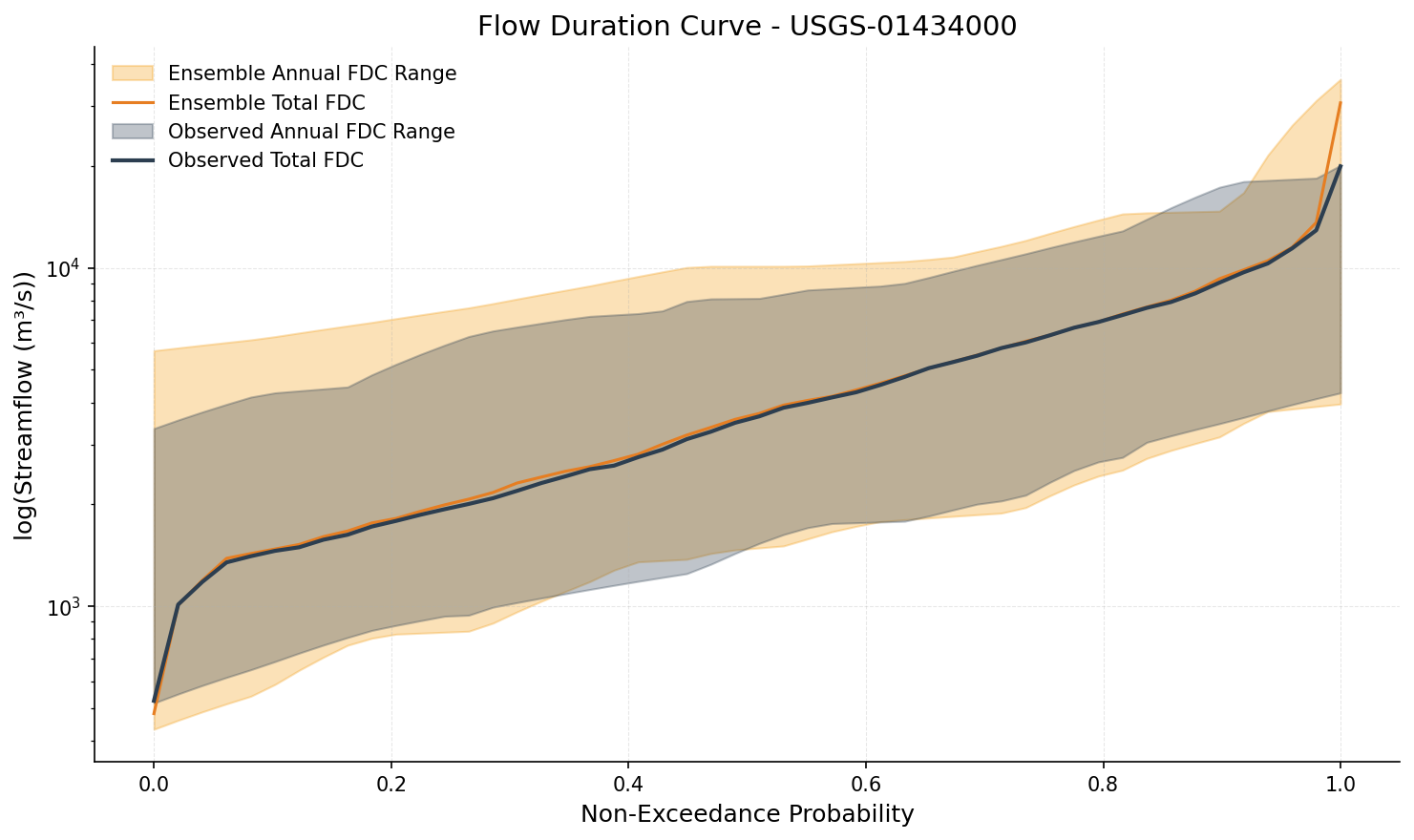
Pass show_annual_range=False to drop the per-year FDC envelope and keep
only the cross-realization band.
Monthly distributions
plot_monthly_distributions is the standard seasonality diagnostic. Side-by-side
boxplots compare ensemble and observed flows, separated by month.
fig, ax = plot_monthly_distributions(
    ensemble,
    observed=Q_monthly[site],
    site=site,
    plot_type="box",
)
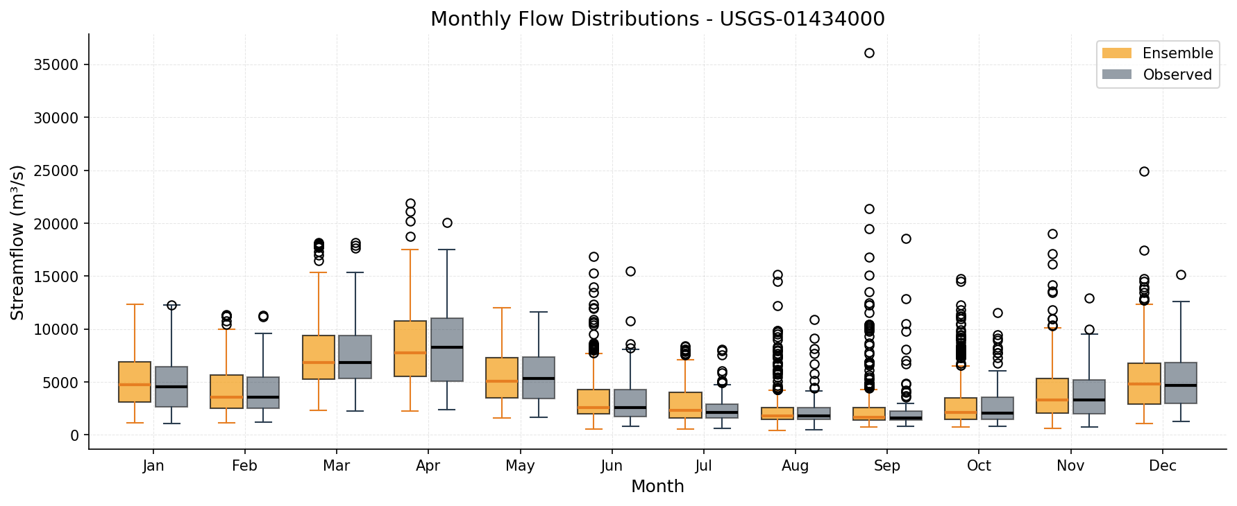
Pass plot_type="violin" for kernel-density violins instead of boxplots.
Validation panel
plot_validation_panel produces a 5-panel summary covering monthly
boxplots, mean and standard-deviation bias, and Wilcoxon and Levene
p-values per month. The observed argument is optional. If you omit it,
the panel falls back to ensemble-only diagnostics.
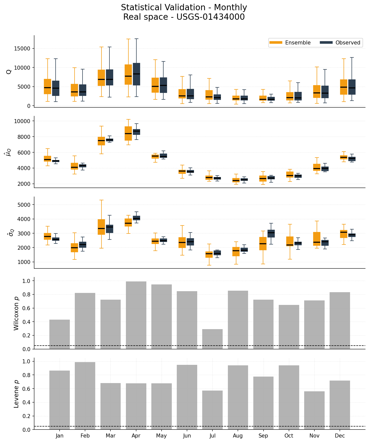
Set log_space=True to run the comparison on log-flows, which can reveal
low-tail differences that the linear-space view hides.
Re-theming
Colors, line widths, and other defaults live in COLORS, STYLE, and
LAYOUT dicts in synhydro.plotting. Mutate them in place and call
apply_plotting_style() to push the changes into matplotlib's rcParams,
and every subsequent plot will pick them up.
from synhydro.plotting import COLORS, apply_plotting_style

COLORS["ensemble_fill"] = "#1f77b4"
COLORS["ensemble_median"] = "#0b3d91"
apply_plotting_style()

fig, ax = plot_timeseries(ensemble, observed=Q_monthly[site], site=site)
This is the simplest way to restyle every figure in a script without threading explicit color arguments through each function call.
Where to find more
- Plotting API reference lists every public function with full argument tables.
- For drought-specific plots, see Tutorial 04.
- For the validation metrics that pair with
plot_validation_panel, see Tutorial 05.
Previous: Ensemble Validation